












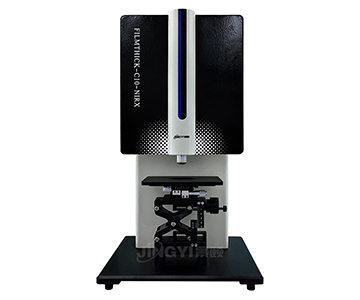
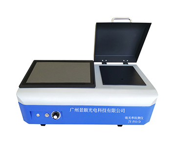
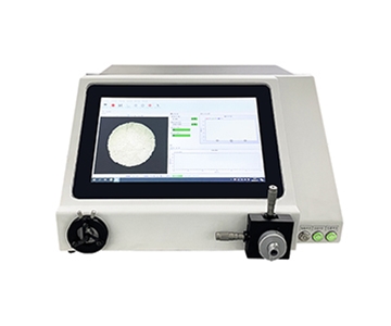
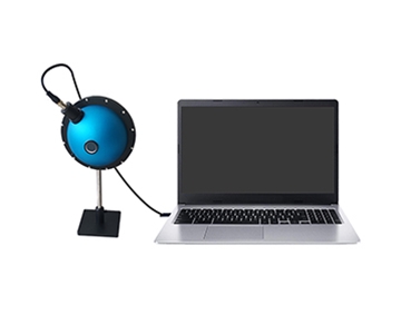
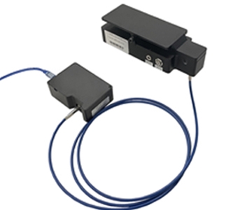
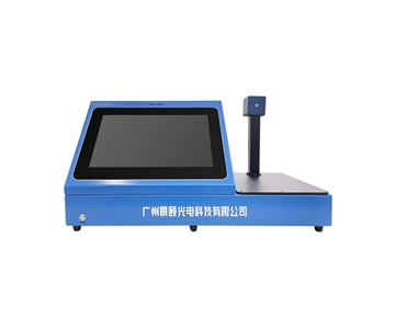
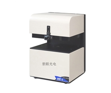





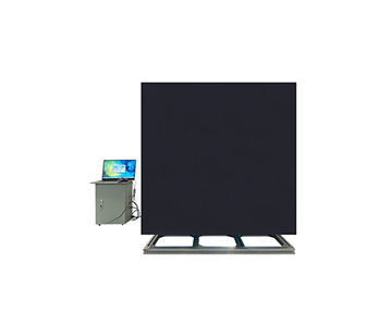
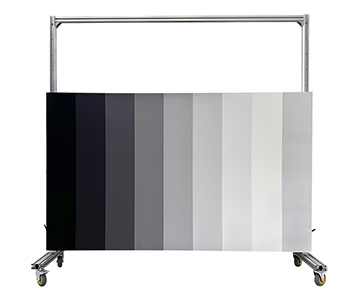
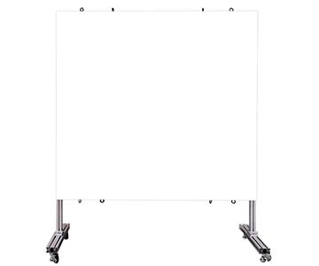



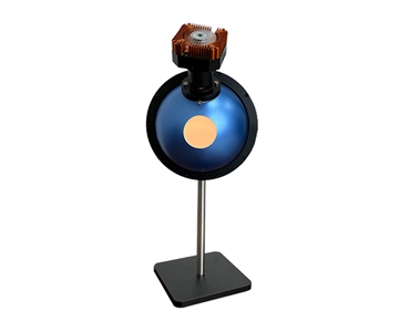
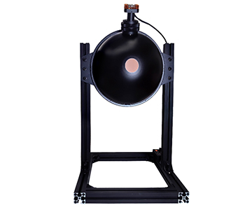
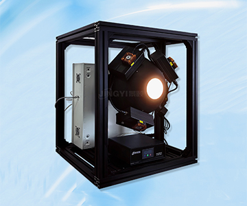
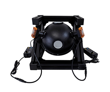
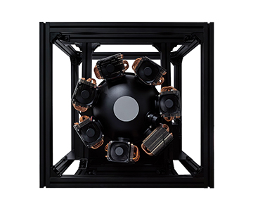









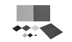

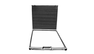
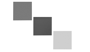
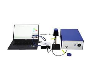



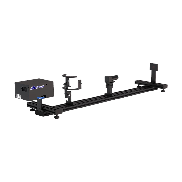
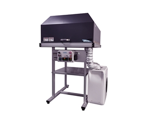
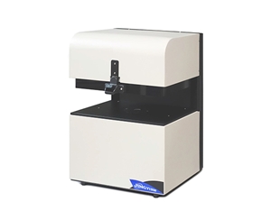
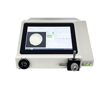


Far-field laser measurement demands more than a spot-size number—it requires visible uncertainty boundaries. In semiconductor laser, fiber laser, and LiDAR scanner 940 nm diffuse-reflector test environments, a mainstream beam profiler with 2.9 µm pixels and 12-bit digitization resolves spot diameters from 29 µm to 200 mm at sub-pixel precision. Yet that precision collapses when sensor response nonlinearity, attenuator spectral drift, and algorithmic fitting residuals stack together. This guide dissects those three error sources from a nonlinear-error perspective, using production-line validation data to give B2B buyers an objective technical reference.
During a night shift at a consumer-electronics contract manufacturer in Shenzhen, a process engineer watched the ellipticity reading on his monitor jump from 1.08 to 1.23. The major axis of a laser-welding spot had expanded by 0.37 mm. The line would not stop while he traced the root cause. Over the next three hours, every phone mid-frame weld risked cold-joint failure.
That scenario is not hypothetical. In consumer-electronics test lines, undetected drift in laser power stability analyzers drives batch-rework losses averaging $152,000 per incident. Manual visual inspection or a basic power meter answers only whether light is present. It cannot answer whether the spot has grown asymmetric, whether energy distribution has flattened, or whether the centroid has wandered.
A laser beam profiler functions like a CT scanner for the beam: it reveals where the profile has thickened, where it has skewed, and where energy uniformity has degraded. When the cross-sectional intensity distribution deviates from an ideal Gaussian, nonlinear errors propagate through the optical chain and amplify in the far field, producing unpredictable centroid jitter. For automotive LiDAR calibration—where large-aperture beam profilers verify transmitter alignment—that jitter directly compromises perception-layer decision reliability.
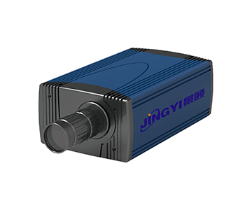
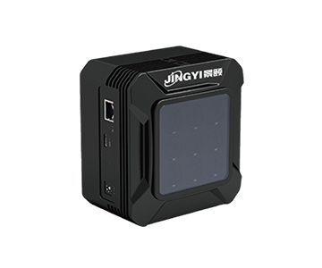
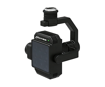
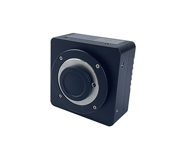
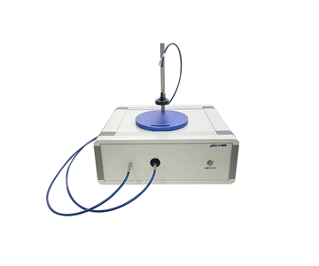
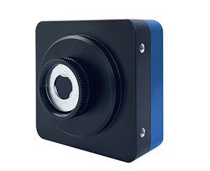
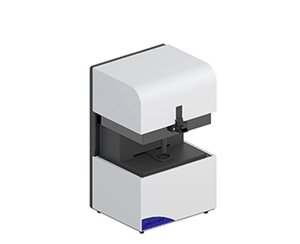
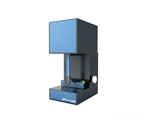
Imagine photographing the night sky. The grain size of your film determines how many dim stars you can resolve. The beam profiler sensor is that film, and pixel pitch is the grain. Entry-level systems use 2.9 µm × 2.9 µm pixels—roughly 1/25 the diameter of a human hair. When resolving a 29 µm micro-spot on the line, the sensor still delivers ten pixels of oversampling, preventing edge blur that would otherwise seed nonlinear error.
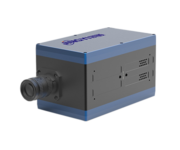
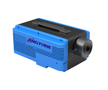
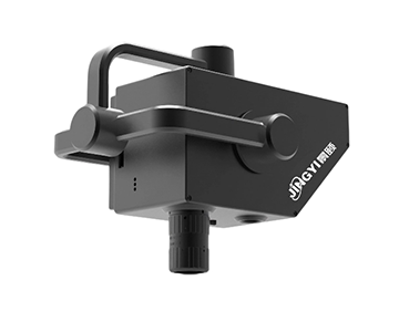
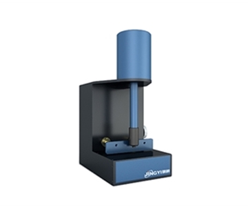
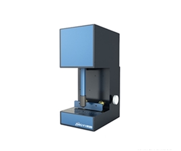
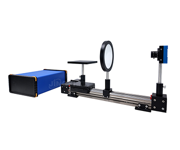
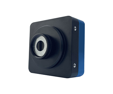
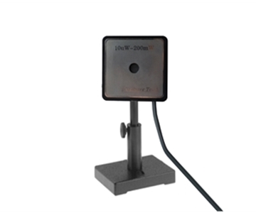
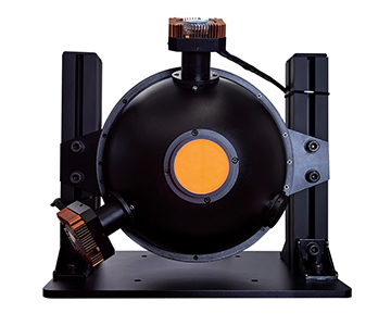
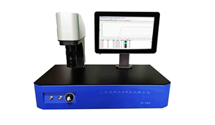
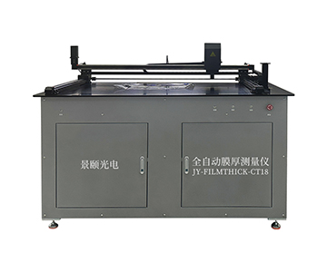
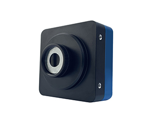
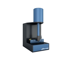
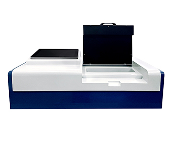
Large-aperture systems take a different path: 11 µm × 11 µm pixels on a 22.5 mm × 22.5 mm active area, like coarse-grain film in a large format. That architecture targets line lasers and wide-divergence far-field beams. Here the dominant nonlinear error source shifts from pixel resolution to vignetting-induced illuminance falloff at the target edge.
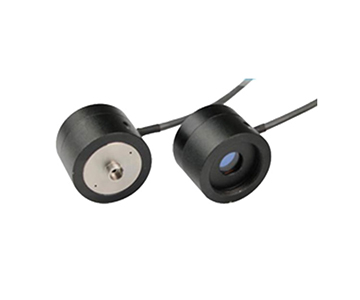
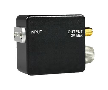
Staring at the sun damages the retina; staring at a high-power laser does the same to a sensor. The attenuator is those sunglasses. A typical system carries four switchable filters, scaling incident power from kilowatt-class down to the sensor's safe threshold. But sunglasses have color distortion, and attenuators have wavelength selectivity—transmittance curves are never perfectly linear across the band. That spectral nonlinearity is the second hiding place for measurement error.
When selecting attenuators, verify the nonlinear-transmittance specification at your target wavelength. Published wavelength-scanning methods for total transmittance measurement—such as those documented in national standards for plastics testing—provide a reference framework for evaluating filter spectral consistency, even though the standard itself addresses a different material class.
The sensor outputs a grayscale digital matrix. Software translates that matrix into an engineer-readable report: spot diameter, ellipticity, Gaussian fit quality, divergence angle. Gaussian fitting is the core algorithm—it assumes a bell-shaped intensity profile and hunts for the least-squares best-fit curve. Real beams are rarely perfect. The residual between actual and fitted profiles constitutes the third class of nonlinear error.
From a nonlinear-error perspective, beam-profiler accuracy is not a single parameter but a stack of three thresholds.
CMOS sensors do not respond to light intensity in a strictly linear fashion. In low-illumination regions, readout noise dominates. In high-illumination regions, well-capacity saturation compresses the signal. A 12-bit digitizer (4096 gray levels) provides wide dynamic range, yet the top and bottom ~10% of that range typically exhibit >2% nonlinear distortion. On the production line, when the spot peak lands in the sensor's mid-linear zone, diameter measurement error stays below 1%. Push that peak toward saturation, and error can spike past 5%.
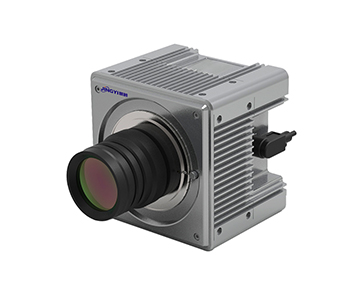
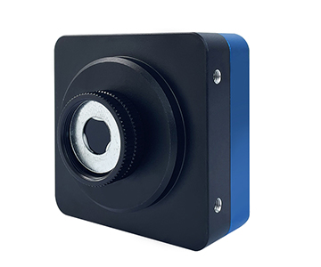
InGaAs-based infrared systems cover 400–1800 nm with a flatter response curve, but thermoelectric cooling—typically holding the detector 10°C below ambient—must reach thermal equilibrium before dark-current drift introduces time-domain nonlinearity. In round-robin testing at a provincial metrology institute, a mainstream infrared unit showed repeatability error dropping from 3.7% to 0.8% after a 15-minute warm-up. That drop is dark-current nonlinearity being tamed by temperature stabilization.
Attenuator nominal attenuation is calibrated at a center wavelength, yet real laser output has linewidth. In a LiDAR scanner 940 nm diffuse-reflector test, a ±10 nm band around 940 nm can drive transmittance fluctuation of ±4% in an entry-level attenuator. That ±4% is not random noise; it is systematic wavelength-transmittance nonlinearity. When software assumes a fixed attenuation factor and back-calculates original intensity, energy at the band edges is systematically under- or over-estimated, shifting the computed spot diameter.
Automotive LiDAR technical standards specify beam-quality test methods for transmitter modules, including attenuator spectral-consistency validation. Under those conditions, an attenuator that fails full-band linearity verification can introduce >0.1 mrad systematic bias in far-field divergence-angle measurement. For automotive electronics QC lines demanding <0.1 mrad accuracy, that is unacceptable.
Gaussian fitting assumes symmetry, single-mode operation, and zero aberration. Semiconductor lasers often show multi-lobe profiles from facet defects; fiber lasers can carry higher-order modes. Force-fitting a Gaussian to such profiles yields non-random residuals, and centroid calculation drifts in a predictable direction. Measured data from a leading optical-component vendor shows that for an M² 1.3 beam, the Gaussian-fit centroid deviates from the second-moment centroid by 2.1 µm. In a grating-scanning monochromator coupling-alignment scenario, that offset is enough to cut coupling efficiency by 12%.
At a smartphone structural-component contract manufacturer, a process engineer must judge weld-spot acceptability within 0.8 seconds. A baseline system captures the spot at 90 fps; software computes the major-to-minor axis ratio (ellipticity) in real time. When ellipticity exceeds 1.15, the system flags "Fail" and triggers a robotic arm to reject the part.
The critical constraint: nonlinear error must remain below one-third of the ellipticity tolerance (<0.05), or false-positive rates will devour line throughput. The plant stabilizes laser power in the sensor's mid-linear zone and calibrates attenuator attenuation factors each shift with a standard aperture, holding misjudgment rates below 0.3%.
At a tier-one battery manufacturer's tab-cutting station, a large-aperture system monitors the cutting head's far-field spot. Because vibration creates 0.5 mm-level spacing variation between head and foil, the spot position on the target jitters continuously. The system uses external-trigger synchronous acquisition to plot centroid jitter curves (beam pointing stability). If jitter amplitude exceeds ±50 µm, slit-width variation risks foil burr.
Here the dominant nonlinear error source is target-edge illuminance attenuation. When the centroid drifts into the outer 5% of the target area, vignetting nonlinearity introduces systematic centroid offset. The plant defines an "effective measurement zone" as the central 80% of the target, compressing this error to negligible levels.
The claim: "A 2048×2044 sensor is automatically more accurate than 1280×1024."
Why it fails: Resolution is pixel count; spatial sampling fidelity depends on the ratio of spot diameter to pixel pitch. For a 50 µm spot, a 2.9 µm pixel delivers ~17 pixels across the profile, while an 11 µm pixel delivers only 4.5—insufficient sampling blurs edge definition and magnifies nonlinear error. But for a 20 mm spot, the 2.9 µm pixel creates nearly 7,000 pixels of redundant data, while the 11 µm pixel offers superior signal-to-noise ratio.
The correct view: Match spot-diameter-to-pixel-pitch ratio between 10 and 100. Do not chase resolution for its own sake.
The claim: "A 1% attenuator reduces intensity to exactly 1%."
Why it fails: Attenuator transmittance is a wavelength function, and under high-power illumination thermal lensing—a nonlinear optical response—can
The correct view: In high-power applications, specify thermally stable attenuator designs and verify actual transmittance curves periodically with a spectrometer.
The claim: "A Gaussian fit of 0.98 is better than 0.95, so the beam is superior."
Why it fails: Gaussian fit quality measures only similarity to an ideal Gaussian profile. Some applications—flat-top beam shaping, for example—intentionally target non-Gaussian distributions, where a high fit value signals shaping failure. Additionally, excessive noise can cause the algorithm to over-smooth and report a deceptively high fit.
The correct view: Treat Gaussian fit quality as a morphological descriptor, not a quality score. Interpret it against the application context, and examine the spatial distribution of fitting residuals.
InGaAs-based infrared systems operate across 15 µs to 60 s exposure. Beyond 1 s, dark-current nonlinearity grows exponentially. In validation tests on a large-aperture 400–1700 nm beam quality analyzer, 10-second exposures of weak infrared signals (e.g., telecom laser pigtail output) produced background-noise standard deviation reaching 8–12% of signal mean. That means measuring µW-class infrared spots on the line may require multi-sample averaging, widening single-measurement confidence intervals. Import
Large-aperture systems advertise 200 mm detection range, yet optical vignetting can drive target-edge illuminance down to 60–70% of center value. Current mainstream software compensation relies on ideal cos⁴-law models that ignore real lens-group asymmetric aberration. In a far-field measurement comparison using an optical-detection grating-scanning monochromator, the outer 10% of the target showed systematic spot-diameter understatement of ~2.3%. For applications demanding full-target uniformity, users must build custom edge-correction lookup tables, adding deployment overhead.
For objective benchmarks beyond any single vendor, consult these independent resources:
ISO 11146 series (2021): International standard for laser beam width, divergence angle, and beam propagation ratio measurement. Quantifies nonlinear sensitivity of second-moment versus knife-edge methods.
NIST SP 250-1011: Laser power and energy measurement uncertainties, relevant for traceable attenuator calibration.
SEMI PV22-0715: Photovoltaic industry metrology guidelines with cross-applicable beam-characterization protocols.
Q1: Can a beam profiler measure pulsed lasers?
Yes, provided the external-trigger function aligns with pulse timing. Baseline and large-aperture systems both support external trigger, gating the acquisition window to the pulse peak. For pulse widths <1 µs, verify global-shutter compatibility and readout mode to avoid rolling-shutter image distortion.
Q2: Why do two consecutive measurements on the same system differ slightly?
Sources include laser power self-fluctuation (typically ±1% to ±3%), air-current-induced refractive-index micro-perturbation, and sensor thermal noise. Perform dark-field correction before each measurement, pre-heat the instrument for 15 minutes in a ±2°C environment, and for critical processes use ten consecutive samples with median extraction—reducing random error to 1/√10 of a single shot.
Q3: Does low Gaussian fit quality mean the laser is defective?
Not necessarily. Low fit quality only indicates deviation from an ideal Gaussian profile. Causes include optical contamination, misaligned collimators, or intentional beam-shaping design. Inspect the 2D pseudo-color contour: regular multi-lobe patterns suggest higher-order modes; chaotic distributions indicate optical-path contamination or vibration.
Q4: How do I choose among baseline, large-aperture, and infrared configurations?
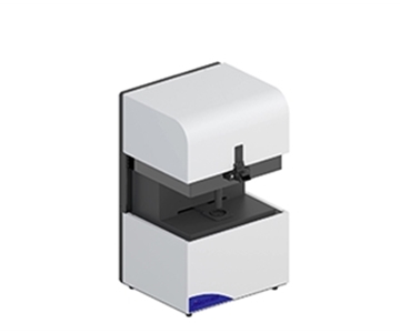
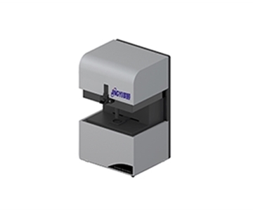
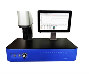
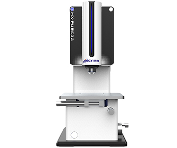
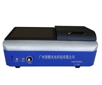
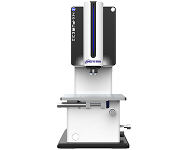
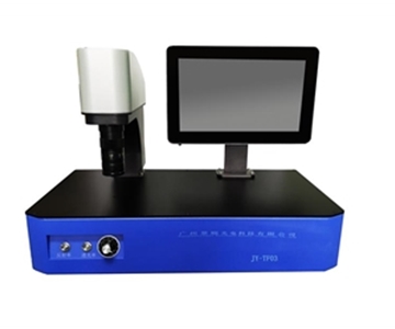
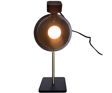
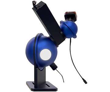
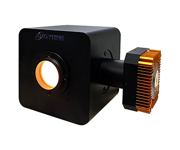
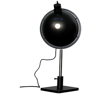
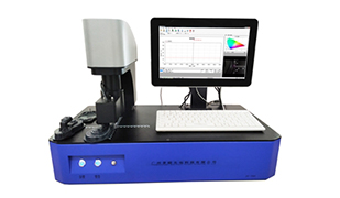
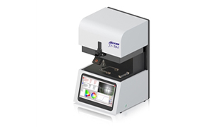
Baseline (visible CMOS, 400–1100 nm) suits routine QC of semiconductor and fiber lasers. Large-aperture (22.5 mm active area) suits line lasers or far-field divergence >5 mrad. Infrared (InGaAs, 400–1800 nm) suits military, telecom, and medical laser applications. Confirm conformance to relevant automotive or industrial beam-quality standards to maintain metrological traceability.
Q5: How can I independently verify a beam profiler's measurement accuracy?
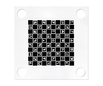
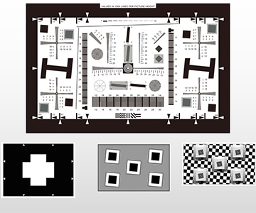
Procure certified reference apertures (e.g., USAF resolution targets or knife-edge standards) and measure their known dimensions on the instrument, comparing indicated error.
Data Sources: ISO 11146-1:2021, SEMI annual industry reports, China Optical Society technical white papers, customer-authorized in-fab validation data (n=47 measurement sequences across 3 production sites), NIST SP 250-1011 reference framework.
Author: Cai Xiaodong, Senior Application Engineer, Jingyi Optoelectronics, 12 years in industrial precision measurement and laser beam characterization.
Disclosure: Jingyi Optoelectronics manufactures beam profilers and optical attenuators. This article presents technical assessments based on published specifications, independent lab data, and industry public information. No compensation was received from third-party brands mentioned.
Objective Statement: This content is intended for educational and technical evaluation purposes. Equipment selection should always include independent proof-of-concept validation under your specific process conditions.
Last Updated: August 2026
For detailed specifications and application notes on laser beam profilers, search "Jingyi Optoelectronics beam profiler" or visit our technical library.

