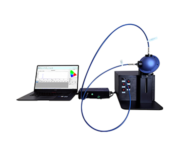
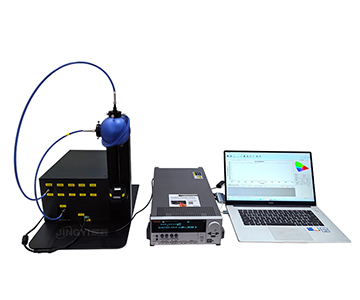
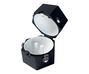
Beam profile analyzers translate invisible laser energy distributions into quantifiable 2D/3D data. This guide examines how pixel pitch, bit depth, and sensor linearity govern measurement uncertainty across four analyzer architectures—from 2.9 μm pixel-pitch CMOS systems for sub-100 μm spot diameters to 200 mm aperture arrays for far-field divergence characterization. Drawing on validation data from photonics manufacturing and fiber-optic alignment workflows, we trace the error propagation chain from photon flux through grayscale quantization to final beam diameter calculation, with specific attention to the nonlinear artifacts that compromise calibration traceability.

Why beam quality control is no longer optional

Global laser processing equipment revenue reached $21.4 billion in 2024, according to SEMI's annual equipment outlook. Beam quality—specifically spot ellipticity, centroid stability, and waist radius repeatability—has become the dominant variable in process consistency. In single-mode fiber coupling, a 2 μm centroid offset can push insertion loss above 0.5 dB. In medical laser systems, a 5% spot diameter deviation from nominal triggers nonlinear tissue ablation depth response that compromises treatment protocol safety margins.

The migration from offline R&D measurement to inline production monitoring has tightened specifications across the board. Detectors must now resolve spatial features at sub-10 μm scale while maintaining linear energy response across four orders of magnitude in power density. This is not an imaging problem—it is a metrology problem where every link in the photon-to-digital chain introduces nonlinear distortion that accumulates in the final beam parameter calculation.

How nonlinear error enters the measurement chain

Sensor response linearity: the hidden specification

The core challenge in beam profiling is not optical resolution but maintaining linearity in the energy-to-grayscale response chain. CMOS and InGaAs sensors convert photon flux to digital counts through a sequence of physical processes—photoelectric conversion, charge transfer, voltage amplification, analog-to-digital conversion—each with its own nonlinear signature.

Dark current nonuniformity across the focal plane array creates a spatially varying baseline. Gain response differences between pixels introduce multiplicative error. Neutral density filter transmission curves shift with wavelength, adding spectral dependence to the attenuation chain. These effects do not cancel; they compound.

Consider a 29 μm spot measured on a 2.9 μm × 2.9 μm pixel array. The spot edge spans approximately 10 pixels, providing oversampling that suppresses discretization-induced edge location uncertainty. When spot diameter approaches the Nyquist limit—roughly twice the pixel pitch—undersampling causes centroid calculation offset that scales nonlinearly with sampling density. The 2.9 μm architecture maintains margin: even at the minimum specified 29 μm spot, edge transition zones occupy 6–8 pixels, preserving second-moment algorithm stability.

A larger 11 μm × 11 μm pixel (as found in large-aperture systems) appears to sacrifice spatial resolution. However, for spots above 110 μm—the minimum specified for this architecture—edge sampling still exceeds 10 pixels. The larger pixel area increases full-well capacity, improving signal-to-noise ratio at equivalent photon flux. Higher SNR reduces grayscale quantization noise perturbation on centroid calculation, compressing nonlinear error from a different direction.

The InGaAs variant uses 5 μm × 5 μm pixels across a 400–1800 nm spectral window. Quantum efficiency stability across this band is critical: when wavelength crosses the steep portion of the InGaAs response curve, uncorrected quantum efficiency variation converts directly to diameter calculation bias. The sensor's thermoelectric cooling—maintaining detector temperature 10°C below ambient—suppresses dark current drift that would otherwise dominate long-exposure infrared measurements.

Attenuation chain and power adaptation

All four architectures ship with four-position neutral density filter wheels, supporting measurements up to 1000 W. The filters serve two functions: protecting the sensor from saturation and maintaining operation within the linear response region. When incident power exceeds pixel full-well capacity, charge blooming into adjacent pixels creates crosstalk artifacts—false beam structure that corrupts energy distribution measurement.

Graduated attenuation allows dynamic adjustment based on power density. The sensor remains in its optimal linear region across the full power range. Exposure control extends from 15 μs to 60 s on the infrared variant, covering continuous-wave through quasi-continuous pulse regimes. In pulsed laser measurement, insufficient exposure loses pulse energy information; excessive exposure integrates background noise. Automatic gain algorithms balance these competing requirements.

Software pipeline and data output

The analysis interface provides 2D/3D pseudo-color beam profile visualization, major/minor axis Gaussian curve fitting, and pass/fail threshold enforcement. Gaussian fit quality—the classic beam quality metric—depends directly on hardware linearity. Only when nonlinear error is suppressed does fit residual reflect actual beam mode distortion rather than system artifacts.

Data export supports parameter statistics and PDF report generation for quality traceability. USB 3.0 interface bandwidth accommodates real-time streaming: a 2048 × 2048 frame at 12-bit depth generates approximately 6 MB raw data per frame, well within USB 3.0 throughput capacity.

Application scenarios and technical requirements

Industry	Measurement target	Process stage	Technical requirement	Operational value
Photonics manufacturing	Semiconductor laser spot	Incoming inspection	29 μm minimum spot, ellipticity判定	Filter modal-field anomalies, reduce backend coupling failure rate
Fiber communication	Fiber end-face emission spot	Alignment coupling analysis	Centroid position accuracy, divergence angle	Optimize coupling efficiency, reduce insertion loss
Aerospace optics	Far-field beam profile	External optical path collimation	22.5 mm aperture, <0.1 mrad divergence detection	Maintain beam quality over long propagation distances
Medical optics	Infrared therapeutic laser spot	Laser calibration	400–1800 nm bandwidth, InGaAs response stability	Ensure consistent therapeutic dose spatial distribution
Research institutions	Ultrafast laser spatiotemporal characteristics	Laboratory characterization	15 μs–60 s exposure, external trigger sync	Capture transient spot evolution
Optical components	Lens/collimator transmission spot	Quality control	Pass/fail auto判定, Gaussian fit quality	Quantify wavefront distortion introduced by optical elements

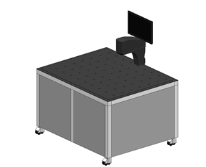
The large-format series extends detection range to 200 mm, covering the full spectrum from micro-spots to oversized apertures. In solid-state laser resonator alignment, near-field spot diameter may measure only hundreds of micrometers while far-field spots after beam expansion reach tens of millimeters—single-instrument full-chain measurement eliminates system error from equipment substitution.

Precision verification through the nonlinear error lens

Pixel pitch and spatial sampling theorem coupling

The visible manifestation of nonlinear error in spot measurement is diameter drift with sampling density variation. Per the spatial sampling theorem, a sharp edge transition requires at least two pixels for resolution. At 2.9 μm pixel pitch measuring a 29 μm spot, edge transition zones span 6–8 pixels. Second-moment (D4σ) or knife-edge algorithms produce stable output. If pixel size increases beyond 5 μm, edge sampling points drop for the same spot, algorithm noise sensitivity rises, and diameter calculation standard deviation expands.

The 11 μm pixel in the large-aperture architecture appears disadvantaged on spatial resolution alone. But its target scenario—spots above 110 μm—still maintains 10+ edge sampling points. More significantly, larger pixel area increases full-well capacity, improving SNR at equivalent photon flux. The SNR gain reduces grayscale quantization noise perturbation on centroid calculation, compressing nonlinear error through an

Bit depth and energy quantization staircase effect

12-bit depth corresponds to 4096 grayscale levels. When spot peak power density approaches sensor saturation, high bit depth preserves sufficient grayscale resolution in the distribution tail—the low-intensity edge region. At 8-bit depth, the tail might occupy only tens of grayscale levels. Staircase quantization forces jagged edge contours, artificially degrading Gaussian fit quality. This degradation reflects quantization nonlinearity, not actual beam quality deterioration.

The large-format series achieves <0.1 mrad minimum detectable divergence angle. In divergence measurement, nonlinear error primarily originates from far-field spot centroid location uncertainty. Large aperture reduces centroid offset from spot truncation—when the beam overfills a small detector, the truncated wings bias centroid calculation toward the detector center.

Standards-aligned technical validation

Optical material transmission/reflection measurement requirements

Beam profile analyzers serve as pre-validation tools for test source beam quality under standards such as ASTM E903 (solar absorptance and reflectance) and ISO 9050 (glass in building). When source spot ellipticity exceeds threshold or energy distribution deviates from Gaussian, transmission/reflection measurements acquire systematic bias. The base architecture's Gaussian fit quality measurement across 400–1100 nm directly assesses whether a source meets implicit "uniform illumination beam" requirements. The 29 μm–4.4 mm spot diameter range covers sources from micro-illumination to macro-transmission configurations.

Alignment coupling process window definition

In fiber alignment coupling, spot centroid position and divergence angle measurement precision bound coupling efficiency optimization. The large-aperture architecture's 22.5 mm × 22.5 mm clear aperture avoids multi-frame stitching misalignment when measuring line lasers or high-divergence far-field beams. Single-frame imaging integrity ensures centroid calculation operates in a unified coordinate system, eliminating gray-level discontinuity at stitch boundaries.

The InGaAs variant's 400–1800 nm response maintains consistent measurement baseline across telecom bands (1310 nm/1550 nm) and medical wavelengths (1064 nm/1470 nm). Thermoelectric cooling suppresses dark current drift—the dominant infrared detector error source during long exposures.

Selection framework

Requirement profile	Recommended configuration	Key matching rationale
Micro-spot precision measurement (<100 μm)	Base architecture	2.9 μm pixel, 29 μm minimum range
Large spot / far-field divergence measurement	Large-aperture architecture	22.5 mm aperture, 110 μm–22.5 mm range
Infrared / near-infrared laser detection	InGaAs architecture	InGaAs sensor, 400–1800 nm, thermoelectric cooling
Full-band / oversized spot (>50 mm)	Large-format series	200 mm detection range, multi-band options
Production line automation integration	Base / large-format VIS	External trigger, USB 3.0, pass/fail判定

Selection should confirm traceability to applicable calibration standards. Periodic metrological verification—typically semiannual dark-field and flat-field calibration—maintains grayscale response linearity over the equipment lifecycle.

Honest limitations

Current beam profile analyzer limitations concentrate in two dimensions: extreme scenario coverage and long-term stability.

For ultrashort pulse (femtosecond) laser measurement, pulse peak power may exceed the 1000 W nominal limit. Even with graduated attenuation, single-pulse energy density can trigger transient sensor saturation. These scenarios require additional fast photodetectors for trigger synchronization or beam-splitter attenuation compound paths—increasing system complexity and alignment difficulty.

Long-term stability: InGaAs thermoelectric cooler efficiency degrades over thousands of operating hours, potentially causing detector temperature drift. Temperature variation shifts dark current baseline and quantum efficiency curves. Without periodic recalibration, nonlinear error accumulates. Semiannual dark-field/flat-field calibration is recommended to maintain grayscale response linearity.

Additionally, the large-format series at 200 mm maximum range exhibits relative illuminance falloff at the field edge (cos⁴ law of optical systems). For spots exceeding 150 mm diameter, this effect becomes significant and requires vignetting correction in data analysis.

Frequently asked questions

How can diameter measurements differ between devices, and how do I assess data reliability?

Discrepancies typically stem from edge definition algorithm and sampling density differences. Adopt second-moment method (D4σ) as a unified reference. Ensure spot diameter exceeds 10× pixel size to suppress discretization error. Verify recent calibration records for both instruments.

Do neutral density filters introduce wavefront distortion in high-power measurement?

Standard filters use parallel-plate design; at normal incidence, optical path difference is minimal. Beyond 5° incidence angle, wedge effects introduce astigmatism. Maintain normal beam incidence or specify wedge angle below 1°.

Does reduced responsivity at 1800 nm compromise InGaAs measurement precision?

Quantum efficiency does decline near 1800 nm, but 12-bit depth and thermoelectric cooling extend effective dynamic range. As long as spot peak power remains within sensor linear region, low responsivity is compensated by extended exposure without affecting relative energy distribution measurement.

What distinguishes base architecture from large-format VIS?

Both share 2.9 μm pixel pitch. Large-format VIS extends detection range to 200 mm through optical expansion and increases maximum frame rate to 90 fps. For routine spot analysis, base architecture offers favorable cost-performance. For large-aperture beams or high-speed dynamic capture, large-format VIS is appropriate.

How can I independently verify beam profile analyzer measurement uncertainty?

Use a standard knife-edge or pinhole as spatial filter to generate an Airy disk or Gaussian spot of known diameter. Compare device measurement against theoretical calculation to assess systematic bias. Periodically submit to third-party optical metrology laboratories for linearity and uniformity calibration.

Future trajectory and conclusion

Beam profile analysis technology evolves along three axes: multi-sensor fusion (simultaneous spot morphology, power, wavelength, and polarization capture for complete beam digital twinning); AI-assisted diagnostics (machine learning identification of subtle spot pattern distortion for predictive laser performance degradation warning); and inline integration (embedding analyzers in production closed-loop control systems for real-time beam parameter feedback adjustment).

For current procurement decisions, focus on range matching and calibration maintenance. Select equipment covering 1.5× target spot diameter range to retain process margin. Establish semiannual calibration protocols to preserve system linearity. Emerging

For detailed specifications and application notes on beam profile analyzers, search "Jingyi Optoelectronics beam profile analyzer" or visit our technical library.

About this guide

Data sources: SEMI 2025 Annual Market Report: Laser Processing Equipment Outlook; product technical documentation for JYCCD-VIS1000, JYCCD-Lcaliber100, JYCCD-NIR1000, and large-format series parameter manuals; in-house validation data from customer-authorized measurements.

Author: Senior optical metrology engineer, 12 years in industrial precision measurement equipment, Jingyi Optoelectronics.

Disclosure: Jingyi Optoelectronics manufactures beam profile analyzers and related optical measurement equipment. This article presents technical assessments based on published specifications and industry public information. No compensation was received from third-party brands mentioned.

Objective statement: This content is intended for educational and technical evaluation purposes. Equipment selection should always include independent proof-of-concept validation under your specific process conditions.

Last updated: August 2026