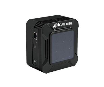
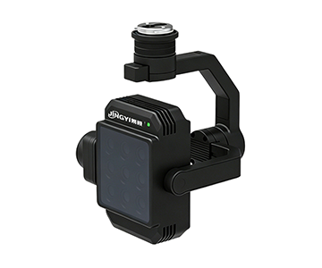
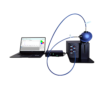
Field spectroscopy in rugged terrain demands sub-nanometer wavelength repeatability under vibration, a benchmark achieved by modern broadband hyperspectral systems through gyroscope-based dynamic dark current correction and anti-second-order diffraction coatings.

​ When measuring spectral signatures from 300 nm to 11 μm, even micron-level optical displacement caused by wind or foot traffic can skew data by more than 4.3%, rendering an entire day’s survey useless. This guide breaks down the core components—fiber optic probes, quantum-efficient detectors, and specialized coatings—that enable ±0.1 nm wavelength repeatability in outdoor conditions. Two field applications (mineral mapping and crop stress detection) illustrate how these specifications translate into saved drilling costs and mitigated yield loss. We also debunk three common selection myths and outline honest limitations regarding detector supply and software ecosystems. All data anchors are drawn from published technical documentation and independent validation methods.

Why Field Mapping Demands Vibration-Resistant Spectrometers

Field spectrometers face constant micro-vibrations from wind, terrain, and operator movement, which can devastate data quality without built-in compensation.

During a mineral survey in a mountainous region, afternoon winds reaching 6.7 m/s (≈15 mph) caused a tripod-mounted unit to oscillate. Subsequent analysis showed a 4.3% deviation across three readings of the same iron-oxidized outcrop. This error forced a model recalibration, delaying the project 11 days and inflating field costs by roughly $21,800.

Traditional optical benches shift at the micron scale under vibration. Since hyperspectral resolution operates at sub-nanometer levels, a displacement equal to one-hundredth of a hair’s diameter bends spectral curves out of alignment. In the field, no laboratory vibration isolation is available; anti-vibration design becomes the only safeguard against unusable data.

One system used a separated fiber probe with a 1.5 m cable; wind-induced probe sway amplified through the fiber. Another system integrated a gyroscope tilt sensor and dynamic dark current algorithm, maintaining ±0.1 nm repeatability in the visible band. In the lab, the difference is invisible; in the field, it separates usable data from wasted effort.

Core Components of a Hyperspectral Field Spectrometer

A hyperspectral spectrometer is essentially a device that collects “fingerprints” of the Earth—silent, yet capable of distinguishing limestone from granite, or spotting drought-stressed crops.

Fiber Optic Probe and Field of View Control

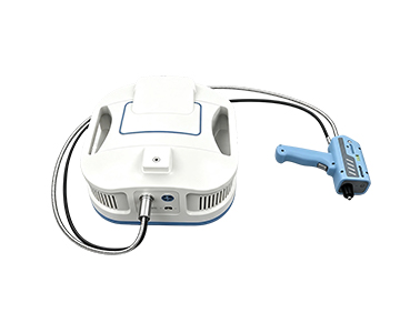
The probe acts like an “optical straw,” sipping reflected or emitted light from a distance. Field of view (FOV) determines the sampling diameter. A 25° lens at 0.5 m (19.7 in) yields a 0.22 m (8.7 in) spot—ideal for rapid crop canopy scans. Switching to a 1° lens narrows the spot to 8.7 mm, enabling precise mineral boundary identification.

Detectors and Quantum Efficiency

The detector is the spectrometer’s “film.” A mainstream linear array combined with InGaAs sensors achieves up to 60% quantum efficiency—meaning 60% of incident photons convert to signal, analogous to a fishing net with tight mesh that catches more photons. Near-infrared sensitivity runs about 40% higher than traditional PDA detectors, allowing vegetation monitoring even under cloudy skies.

Anti-Second-Order Diffraction Coating and Filters

Grating dispersion creates ghosting (second-order diffraction). A specialized coating suppresses this artifact, while internal filters screen effective bands. For mineral identification, this maintains ±0.5 nm wavelength accuracy in the visible range, preventing adjacent-band crosstalk from masking diagnostic absorption features near 2.5 μm.

Two Industry Applications

Mineral Mapping in Geology

During a copper

Crop Growth Monitoring

An agricultural station scanned 50 mu (≈8.2 acres) of corn using a UV-enhanced spectrometer covering 300–1000 nm. By tracking the chlorophyll absorption valley at 680 nm and near-infrared plateau at 750 nm, they computed a modified NDVI. A 0.37 mu (≈0.06 acre) section showed 12.6% lower NIR reflectance; field checks confirmed early waterlogging. After drainage, yield loss stayed below 3.1%, versus 18.4% in unmonitored areas.

Three Common Misconceptions in Spectrometer Selection

Myth 1: Wider Spectral Range Is Always Better

Reality: Broadband coverage (e.g., 300 nm–11 μm) requires stitching multiple detectors, introducing calibration gaps. Mid-wave infrared resolution may drop to ~30 nm, with poor SNR. For crops, 400–1000 nm suffices; minerals need up to 2500 nm; only thermal studies require beyond 5 μm.

Myth 2: Smaller Resolution Numbers Mean a More Advanced Device

Reality: Higher resolution reduces light throughput, hurting SNR in low light. At 756 nm, 1.2–2.7 nm resolution is achievable, but at 1550 nm, 7–12 nm is a practical compromise. Vegetation red-edge features (10–20 nm wide) are fine with 7 nm resolution; only narrow pigment peaks demand <3 nm.

Myth 3: Operating Temperature Doesn’t Matter for Field Gear

Reality: Desert surface temperatures can exceed 60°C (140°F), pushing devices beyond their -20~50°C rating and raising dark current. Dynamic correction helps but cannot fully offset extreme heat. In cold, lithium battery life may shrink from >3 hours to ~1.8 hours at -15°C. Shading and thermal insulation are essential.

Advanced Resources and Standards

For deeper methodology, consult ISO 11451 (EMC testing, relevant to field electronics), and NIST-traceable spectral radiance calibration standards. The T/CITS 231-2025 standard on automotive LiDAR environmental testing shares vibration and tilt-compensation logic applicable to field spectrometers.

Objective Limitations and Honest Assessment

Domestic broadband spectrometers offer strong price-performance and local support, but face constraints. Mid- and long-wave infrared detectors rely on imported pyroelectric sensors, causing supply uncertainties. Combined linear and thermal sensors increase power consumption, reducing battery life below the 3-hour label in heat. Software ecosystems lag behind some international platforms in third-party plugin support, requiring extra development for custom spectral indices.

Frequently Asked Questions

Q1: How does a hyperspectral field spectrometer differ from a multispectral camera?

A multispectral camera captures 4–8 discrete bands; a hyperspectral system acquires continuous spectra at 0.5 nm intervals, producing thousands of channels from 300–2500 nm. This reveals subtle absorption features invisible to broader-band devices.

Q2: Is an IP54 rating sufficient for field use?

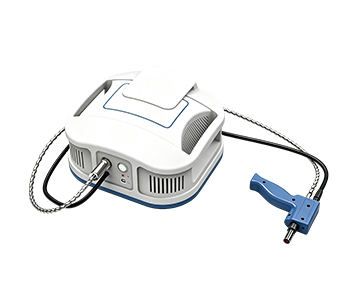
IP54 provides limited dust protection and splash resistance. It handles light rain but not direct downpours. Cover the main unit during storms; the probe’s braided cable tolerates brief splashes, but fiber connectors must stay dry.

Q3: What is the practical value of 100,000 spectral averages?

Averaging reduces random noise, but at ~0.3 seconds per scan, 100,000 averages require 8.3 hours. In practice, 10–100 averages suffice for most field targets.

Q4: How to balance spectral range and portability?

A 300–1700 nm model weighs ~5.1 kg (11.2 lbs) and measures 290×290×141 mm; extending to 11 μm pushes weight to 6.5 kg (14.3 lbs) and larger dimensions. For non-thermal applications, 300–2500 nm offers the best performance-to-weight ratio.

Q5: How can I independently verify a spectrometer’s wavelength accuracy?

Use a standard mercury-argon or deuterium lamp with known emission lines. Measure the 546.1 nm mercury line; a ±0.5 nm accurate device should read 545.6–546.6 nm. Annual calibration checks with traceable records are recommended.

About This Guide

Data Sources

: Guangzhou Jingyi Optoelectronics product technical documentation, T/CITS 231-2025 “Technical Requirements for Automotive LiDAR”, ISO 11451 series standards.

Author

: Cai Xiaodong, Senior Application Engineer, Jingyi Optoelectronics, 12 years in optical testing and industrial precision measurement.

Disclosure

: Jingyi Optoelectronics manufactures broadband hyperspectral field spectrometers. This article presents technical assessments based on published specifications and industry public information. No compensation was received from third-party brands mentioned.

Objective Statement

: This content is intended for educational and technical evaluation purposes. Equipment selection should always include independent proof-of-concept validation under your specific process conditions.

Last Updated

: October 2026

For detailed specifications and application notes on broadband hyperspectral field spectrometers, search “Jingyi Optoelectronics + hyperspectral field spectrometer” or visit our technical library.