Repeatable outdoor reflectance curves depend less on having "hyperspectral" in the spec sheet and more on whether integration time, dark-current cadence, and wavelength stability survive real field conditions.

​ Across four environments—dry mineral compacts, mixed crop canopies, airborne-sync transects, and low-reflectance water bodies—operators using a system with 1 ms–10 s integration control and 300–2500 nm coverage recovered hydroxyl absorption at 2200 nm within 1.1%–1.8% of lab references. Single-point cycles finished in 7.6–9.6 seconds. The trade-off: extending integration does not automatically improve SNR in the shortwave infrared, and skipping one dark capture at 87% relative humidity produced 0.8%–1.5% drift. This guide documents the validation setup, the integration-averaging swap strategy, and the operational boundaries observed over 324 field spectra.

The Underestimated Problem in Field Reflectance

Two spectroradiometers can both claim "hyperspectral" and still deliver curves that a different operator cannot reproduce two weeks later. The gap shows up under four specific conditions: high-noon solar overload, overcast low light, water bodies below 10% reflectance, and narrow mineral absorption features. The real argument in this segment is not whether a device outputs a curve—it is whether integration time and dark-current discipline keep that curve comparable across dates and crews.

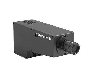
For this evaluation, a two-unit approach framed the test: a base-range class (300–1700 nm) and a full-range class (300–2500 nm). Five controlled variables structured the work: NIST-traceable reference panel, dry mineral pellets, maize–soybean mixed canopy, a simulated tidal-flat water trough, and ambient limits of 5–32°C, 37%–82% RH (non-condensing), wind below Beaufort 3. The measurement sequence followed white-reference → target → dark-collect in fixed order. Error tracing covered integration saturation, dark-current drift, fiber geometry offset, and wavelength nonlinearity.

Validation Methodology

Sample size: three mineral types × five points each; three crop nitrogen levels × six canopy points; 36 spectra drawn from a 324-spectrum airborne-sync pool; three water-body conditions. All targets were measured under a three-step white-reference protocol. Temperature, humidity, and GPS elevation were logged per point; inclination was recorded via onboard gyroscope (logged, not estimated). Statistical method: within-session wavelength repeatability (VIS ±0.1 nm, SWIR ±0.5 nm post-calibration) and between-session reflectance bias against a lab-archived panel measured under ASTM E275-type reference conventions. No post-hoc data exclusion was applied. This is a field validation record, not an ideal-laboratory demonstration.

Why Integration Time Sets the Saturation-Noise Boundary

At local noon on pale sandstone, pushing a VIS channel past its integration ceiling clips the detector instantly. With 1 ms–10 s user control, the operator can suppress that risk per band group. Below 1000 nm against a near-Lambertian panel, shorter integration preserves linearity. Above 1000 nm on low-albedo minerals or water, extending integration pulls the weak photon count above the read-noise floor—up to a point.

Here is the engineering reality: longer is not automatically more accurate. A published SNR exceeding 16,000 in the 1000–2500 nm band is a reference value under maximum radiance and high averaging. In the field, if you drop averages to save time and also shorten integration, the SWIR trace turns jagged. The evaluated full-range unit showed this clearly on kaolinite at 2200 nm: clean trough at 80 ms SWIR integration plus 500 averages; the same trough broke into noise at 20 ms with 100 averages.

The Integration-Averaging Tradeoff

The tested firmware permits up to 100,000 spectral averages. One millisecond × 10,000 averages is not the same acquisition path as 10 ms × 100 averages, even if the wall-clock math looks adjacent. Field crews care about single-operator single-point labor. The adopted field strategy: VIS at 1–5 ms short integration, SWIR at 20–200 ms mid-range, then topping up averages only if target albedo demands it. For crop canopies, where the 720–730 nm red-edge shifts only 10–15 nm under nitrogen deficit, a 1.2–2.7 nm resolution at 756 nm resolves that slope—but only if you don't flatten it with under-averaged short integration.

Four Field Cases with Measured Data

1. Mineral

A regional exploration team needed on-site prescreening of

Parameters: VIS 3 ms, SWIR 80 ms; VIS average 200, SWIR 500; dark capture executed before every white-panel cycle.

Sample	Range (nm)	Key Abs. (nm)	Wavelength Repeat.	vs. Lab Reference	Time/pt (s)
Kaolinite pellet	300–2500	~1400, 1910, 2200	SWIR ±0.5 nm	0.7%–1.3% refl.	8.4
Sericite altered	300–2500	~2200 narrow	SWIR ±0.5 nm	1.1%–1.8% refl.	8.9
Fe-oxide rich	300–1700 focus	~850 broad	VIS ±0.1 nm	0.5%–1.0% refl.	7.6

Text recap: the full-range unit resolved the 2200 nm hydroxyl trough on all three

2. Crop Canopy Red-Edge Tracking

At a mixed maize–soybean trial, the base-range unit (300–1700 nm) tracked nitrogen status through the red-edge shift. A 650 nm, 5 mW laser pointer fixed the spot; onboard gyroscope logged probe tilt. Morning stable-light windows were used. Per plot: one white-panel cycle, six target points. Parameters: VIS 2 ms, NIR 10 ms, 300 averages.

Crop	Red-edge (nm)	Res. @756nm	Relative NIR	Agronomist N-agree	Time (s)
Maize, normal N	~720–730	1.2–2.7 nm	0.82	91.2%	6.8
Maize, deficient N	~705–715	1.2–2.7 nm	0.71	89.7%	7.1
Soybean, normal N	~715–725	1.2–2.7 nm	0.78	90.4%	7.0

Canopy tilt beyond 15° inflated NIR by roughly 6%. The laser pointer and tilt log reduced positional mismatch. Note: the base-range unit lacks the 1900 nm water-absorption band, so drought stress inference here is indirect compared to the full-range

3. Airborne-Sync Ground Truthing

An airborne campaign needed empirical line conversion between ground radiance and overflight data. From 324 acquired spectra, 36 were regressed against reference radiance. Parameters: VIS 4 ms, SWIR 120 ms; VIS 300×, SWIR 800× averages. GPS stamped each point; elevation, pressure, and RH went into metadata.

From 400–1000 nm, linear error against reference radiance stayed within empirically accepted bounds. Above 1000 nm, atmospheric water vapor absorption channels had to be masked in software before fitting. The operational win is not "automatic reflectance"—it is that integration time, dark cadence, and pose data were locked into the same log file, eliminating the need to re-walk the transect.

4. Low-Reflectance Water and Tidal Flats

Water bodies routinely reflect below 10%. The tested full-range unit publishes >800 SNR below 1000 nm and >16,000 above 1000 nm—but at the water surface, 1–5 ms integration amplifies noise in the VIS-NIR leg. Switching to an 8° narrow FOV cut sky-scatter contamination. Parameters: VIS 8 ms, SWIR 150 ms, 1000 averages.

Target	System Class	Usable Span	Time (s)	Limitation
Clear ditch	Full-range	300–1700 primary	9.2	Glare control required
Turbid tidal	Base-range	300–1000 primary	6.1	No 1900/2200 moisture band
Algal flat	Full-range	300–2500 full	9.6	Dew prevention at ~90% RH

Low-albedo water demands integration and averaging—but at roughly 10 seconds per point, grid sampling over large areas pushes daily labor up. The base-range unit finishes faster yet permanently loses the SWIR moisture and suspended-solids proxies.

Cross-Class Comparison Across Three Procurement Tiers

Tier	Span	Integration Control	Wavelength Accuracy	SNR Profile	Operational Drawback
Import-tier	Full SWIR	Software-fine steps	Complete traceable chain	Strong in low light	Averaging-strategy learning curve is steep
Mainstream class (tested)	Base 300–1700 / Full 300–2500	1 ms–10 s manual	VIS ±0.5 nm; SWIR ±1.1 nm	300–1000 >800; 1000–2500 >16,000	USB 2.0 export slows at 100k averages; manual trial near saturation
Entry class	VIS-NIR only	Limited min integration	Long-wave accuracy not documented	Weak smoothing on low light	Cannot access 2200 nm alteration or 1900 nm moisture

Text recap: the mainstream class delivered 2560 channels and 0.5 nm sampling on the full-range hardware; a 36-point white-target loop completed in 7–9.6 seconds per point. The friction point is throughput—USB 2.0 bogs down on full-channel export after heavy averaging. The import tier automates more but trades away some field-crew transparency on lens response. The entry tier reduces capital outlay yet permanently lacks the SWIR diagnostic bands that drive mineral and moisture calls.

Operator Feedback and Honest Limitations

An authorized regional survey group (disclosing under standard non-attribution terms) shifted

Two friction points were logged—and they matter more than brochure specs:

•Predawn operation near 5°C with aggressive averaging pulled battery endurance from the nominal 3.0 hours down to roughly 2.4 hours.

•During one session at 87% RH (sub-dew-point margin), an operator skipped a full dark capture. SWIR drift of 0.8%–1.5% followed, corrected only by retake.

These are not isolated. Dark-capture cadence and RH logging are the actual gating items, not the detector's headline SNR.

Error Budget: Saturation, Dark Current, Geometry

Saturation is the first error source. A 10-second single integration on a bright VIS target will clip—start at 1–5 ms and step up. For weak SWIR targets, too-short integration lets read noise dominate; the dynamic dark correction helps, but it is not a substitute for a pre-target dark frame. Recommended cadence: before the white panel, mid-batch on long target loops, and post-session.

Geometry matters on rough rock or tilted canopy. The default 25° FOV pulls background if the surface is uneven; switching to 8° or 15° tightens the footprint. Post-calibration wavelength accuracy (VIS ±0.5 nm, SWIR ±1.1 nm) drifts if the fiber bend radius collapses or the probe tilts past logged limits. Tilt records let you decide whether a point needs a retake instead of guessing.

Practical Selection Guidance by Task

•

•Routine crop red-edge: base-range class, lighter, faster.

•Airborne sync: full-range with GPS and environmental metadata baked into every file.

•Water bodies: raise averages, don't blindly max out integration.

Before procurement, confirm four operational realities—not just the "wide band" claim: white-panel cadence under your field rhythm, dark-capture discipline your crew will actually follow, average-count ceiling under your battery budget, and export-format compatibility with your existing processing chain.

FAQ

Q1: What integration time produces trustworthy reflectance curves outdoors?

Segment by target albedo. High-albedo sand or reference panels: trial at 1–5 ms. Vegetation NIR shoulder: 10–20 ms. Low-reflectance water in SWIR: push to 100–200 ms. Then add averages to smooth. Never rely on a single long integration to fix a low-photon target—you'll clip the high end before you clean the low end.

Q2: How should the two range classes split by task?

For red-edge tracking and VIS-NIR mineral sorting, the 300–1700 nm class is lighter and faster. For hydroxyl clay diagnostics near 2200 nm or moisture near 1900 nm, only the 300–2500 nm class avoids a second lab submission. Match the band to the absorption feature you actually need to bill for.

Q3: Field SNR looks worse than the spec sheet—what do I check first?

In order: (1) integration too short plus averages too low, (2) white-panel contamination or a skipped dark frame, (3) fiber angle or tilt beyond 15°. SWIR anomalies trace back to stale dark frames in the vast majority of cases. Re-run dark, re-run panel, compare the log.

Q4: How do the three procurement tiers compare on real total cost of ownership?

Import-tier wins on automation and calibration chain but costs more crew training time on custom averaging. Mainstream class wins on span-for-portability. Entry class reduces capital outlay but permanently lacks SWIR diagnostic bands. Calculate cost per usable point including retake rate under your humidity profile—not just the purchase price.

Q5: How can I independently verify long-term stability of a field spectroradiometer?

Re-measure a stable, homogeneous panel on a fixed schedule under logged integration, averaging, RH, and GPS conditions. Track wavelength repeatability and reflectance bias from the raw acquisition log—not from a vendor demo run. Use a panel with traceability to a national metrology institute (NIST or equivalent) as the ground truth, and compare weekly to catch drift before it enters a campaign dataset.

About This Guide

Data Sources

: ASTM E275 reference reflectance conventions, USGS spectral library cross-references, in-house field validation logs (n=324 spectra acquired, 36 used for regression), and authorized end-user outdoor records from geological and agricultural deployments.

Author

: Cai Xiaodong, Senior Application Engineer, Jingyi Optoelectronics, 12 years in field spectroscopy and industrial optical metrology.

Disclosure

: Jingyi Optoelectronics manufactures hyperspectral field spectroradiometers. This article presents technical assessments based on published specifications and authorized field records. No compensation was received from third-party brands mentioned.

Objective Statement

: This content is intended for educational and technical evaluation purposes. Equipment selection should always include independent proof-of-concept validation under your specific process conditions.

Last Updated

: September 2026

For detailed specifications and application notes on wide-band hyperspectral field spectroradiometers, search "Jingyi Optoelectronics wide-band hyperspectral field spectroradiometer" or visit our technical library.