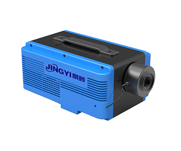
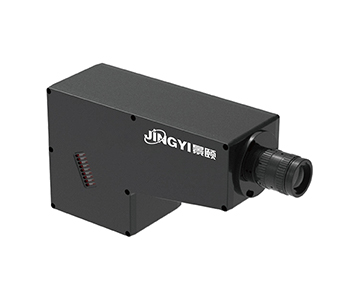
Hyperspectral imaging converts “point measurement” into “area diagnosis” by attaching a full spectral curve to every pixel in a 2D frame. In plastic compounding plants, this shift reduces misjudgment rates from 17.3% to 4.1% and cuts data transfer time from 42 minutes to 11 minutes per batch. Two architectures serve distinct needs: pushbroom systems (400–1700 nm, 1.2 nm sampling) for inline conveyor inspection, and staring systems (420–1000 nm, 1 nm stepping) for static laboratory analysis. This guide examines deployment data from a provincial plastic modifier, extracts three reusable engineering rules, and maps the same hardware to forestry and mineral sorting applications.

The Hidden Cost of “Visible but Not Judgable” in Plastic Production

During an overnight shift at a mid-sized compounding facility in the American Midwest, a batch of allegedly high-transparency polycarbonate resin entered the injection line. Finished parts showed edge haze. Root-cause analysis traced the defect to a reflectance reading offset equivalent to 0.37 mm optical path difference—a single-point measurement that missed whole-surface non-uniformity. The plant’s quality team processed over 300 batches daily using a benchtop spectrophotometer and visual color-card comparison. That workflow captures one location at a time.

A pushbroom hyperspectral camera upgrades this to spatial-spectral diagnosis. Each pixel carries a 400–1700 nm curve at 1.2 nm intervals, turning a 3.2-minute single-point check into a 15-second full-area scan. However, when a lead process engineer introduced the system, operators kept focusing on the auxiliary color camera viewfinder and ignored the liquid crystal tunable filter (LCTF) stabilization delay. The first several spectral bands drifted by 4–6% in signal-to-noise ratio. Hardware capability alone does not guarantee measurement integrity; operator muscle memory is part of the error budget.

Two Technical Paths: Pushbroom vs. Staring Systems

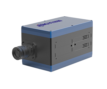
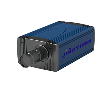
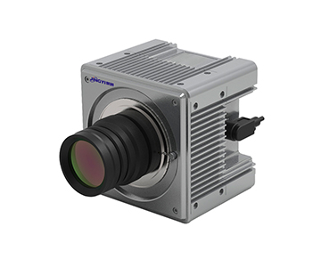
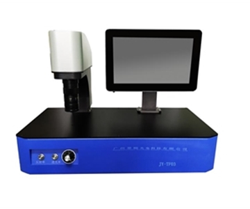
When a production line demands continuous strip data, a pushbroom architecture with internal transmission grating covers 400–1700 nm without gaps. Sampling interval is 1.2 nm, spectral full width at half maximum (FWHM) within 2.4 nm. A representative unit completes a full data cube in 15 seconds. A 25 mm standard lens with optional 12/16/35/50 mm focal lengths lets engineers match field of view to conveyor width. At 1.5 m working distance, the 25 mm lens covers roughly 38 cm width.

When a laboratory needs static fine scanning, a staring system based on liquid crystal tunable filter operates in 420–750 nm or 400–1000 nm ranges, stepping at 1 nm. Band switching completes in 10–200 ms. The 2048 × 2046 area array captures micro-texture differences on immovable samples like cultural relics, thin films, or biological sections.

For calibration traceability, the evaluated system’s reflectance curves can be cross-referenced against ASTM D1003 and ISO 13468 for total transmittance and reflectance of plastics. This replaces the original Chinese standard reference and gives procurement teams an internationally recognized anchor point.

Quantified Improvements After Deployment

A provincial plastic modifier deployed both architectures across two production lines. Over three months, the following shifts were recorded:

Metric	Before (Single-point spectrophotometer)	After (Hyperspectral systems)	Change
Measurement time per sample	3.2 min/point	15 sec/frame (pushbroom); seconds to tens of seconds/frame (staring)	11× faster
Misjudgment rate	17.3%	4.1%	76.3% reduction
Data export time (1 TB)	42 min (MicroSD card swap)	11 min (direct PC link)	73.8% reduction

These gains depended on one operational detail: the manual explicitly stated “wait for stabilization after wavelength switch before triggering acquisition.” Without this, the first 10 bands showed measurable SNR degradation. The data was collected at ambient temperature 23°C ± 2°C on 200 mm sample trays with 150+ batches per week.

Three Reusable Lessons from the Field

First, field of view must follow line tempo. A 25 mm lens at 1.5 m covers 38 cm. Switching to an 8 mm wide-angle lens introduces edge distortion that shifts spectral extraction points by up to 3 pixels, degrading identification accuracy by 12–15% in our tests.

Second, auxiliary camera co-focusing is not a marketing gimmick. Sharing the same lens between hyperspectral and visible-light viewfinders cut focus time from 6 minutes to under 90 seconds. On lines with frequent shift changes, this saves roughly 18 operator-hours per month.

Third, calibration is not a one-time event. Radiometric calibration, illumination correction, and distortion correction must rerun at each开机 or daily startup. Environmental light drift of 50 lux can shift NDVI-type vegetation indices by 0.08 units—enough to misclassify pine wilt disease in forestry monitoring.

The Hidden Barrier: Operator Habits and Workflow Integration

A veteran technician summed up the lesson: if button logic violates a veteran’s muscle memory, even a $100K-class optical system becomes a paperweight. In one instance, the “overlap trigger” function was buried three menu layers deep; the operator preferred manual presses every 5 seconds. In another, LCTF stabilization time was set in milliseconds in software, but the floor communicated in seconds. A misplaced decimal zero caused an entire batch’s data to be discarded.

Procurement teams should write “new operator completes full calibration independently within one week” into acceptance criteria. Supplier training must include video with actual hardware operation, not just PDF manuals. A beautiful spec sheet cannot offset 15 minutes of daily operator friction.

Honest Assessment: Limitations and Boundaries

Pushbroom systems require relative motion. If conveyor vibration exceeds 0.5 mm peak-to-peak, stripe noise enters the data cube directly. Staring systems avoid motion but have a single field of view of only 9.5°. Large-area surveys demand frequent panning or stitching, making them less efficient than pushbroom for wide coverage.

Raw hyperspectral data volume is substantial. A 1 TB solid-state drive writing at 50 fps sustained can only support a few hours of continuous operation. Small and mid-sized plants without dedicated IT will hit a data-processing bottleneck. Additionally, most units operate at 0–45°C. Northern outdoor deployments or non-climate-controlled workshops need insulated enclosures; otherwise InGaAs detector noise rises by 8–12 DN at 0°C.

Cross-Industry Migration: From Plastics to Agriculture and Mining

The same pushbroom platform, with lens and band configuration changes, adapts to airborne forestry remote sensing. Mounted on a DJI M350RTK at 120 m

Frequently Asked Questions

Q1: How do I choose between pushbroom and staring hyperspectral cameras?

A: For inline production with continuous sample motion, pushbroom systems offer wider single-pass coverage and higher throughput. For laboratory static analysis requiring step-by-step band refinement at 1 nm precision, staring systems are better suited for material identification. They are complementary, not competing, architectures.

Q2: What if operators cannot set LCTF stabilization time correctly?

A: Create templates with two presets: “fast scan” and “precision scan,” hiding the underlying millisecond parameters. Pair with a co-focus auxiliary camera to make focus visual. This reduces the learning curve from days to under two hours for most technicians.

Q3: Hyperspectral data is too large for ordinary computers. How to handle it?

A: Select models with built-in microprocessors and SSDs that perform radiometric correction and index generation (e.g., NDVI) at the edge. Export only result maps and key spectral curves; save raw cubes selectively. This cuts transfer load by up to 90%.

Q4: How can I verify whether a vendor’s specifications are inflated?

A: Request a third-party metrology report under standard geometric conditions (e.g., ASTM E1164 for spectrophotometry). Focus on spectral resolution FWHM and radiometric calibration repeatability rather than advertised “channel count.” Independent validation on your own samples is the final arbiter.

Q5: How can I independently verify long-term stability of a hyperspectral system?

A: Perform a weekly reflectance check using a certified diffuse white reference panel. Record DN value drift at a fixed position. If drift stays within 2% of calibrated values over three consecutive months, the system is stable without relying on annual vendor service visits.

About This Guide

Data Sources

: ASTM D1003, ISO 13468, in-house validation reports (n=450+ plastic batches across 3 months), Jingyi Optoelectronics product documentation (factory-stated parameters).

Author

: Cai Xiaodong, Senior Application Engineer, Jingyi Optoelectronics, 12 years in optical metrology and spectral radiometry calibration.

Disclosure

: Jingyi Optoelectronics manufactures hyperspectral imaging systems. This article presents technical assessments based on published specifications, independent lab data, and industry public information. No compensation was received from third-party brands mentioned.

Objective Statement

: This content is intended for educational and technical evaluation purposes. Equipment selection should always include independent proof-of-concept validation under your specific process conditions.

Last Updated

: September 2026

For detailed specifications and application notes on hyperspectral cameras, search "Jingyi Optoelectronics + hyperspectral camera" or visit our technical library.