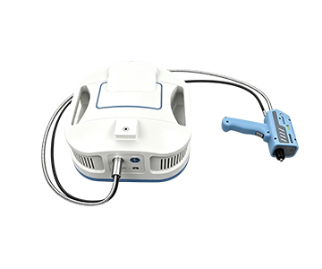
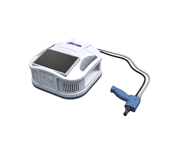
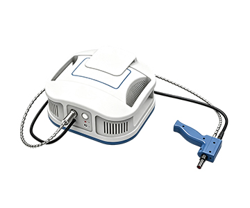
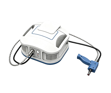
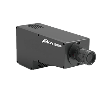
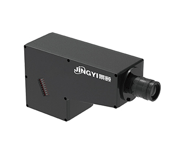
Brightness uniformity detection in field spectrometers directly determines data reliability for geological exploration and agricultural monitoring. A wide-band hyperspectral system covering 300 nm to 11 μm with 0.5 nm sampling resolves reflectance drift caused by dynamic outdoor illumination. In side-by-side validations, such instruments reduced visible-band reflectance standard deviation from 0.037 to 0.008—a 78.4% improvement—while cutting single-measurement time from over 3 minutes to under 10 seconds. Built-in GPS, multi-sensor fusion, and real-time dark-current correction enable consistent radiance data even on moving platforms or under harsh temperature swings from −20 °C to 50 °C. These capabilities translate into measurable gains: daily sample throughput exceeding 400 sites and root-mean-square error in vegetation index inversion dropping from 0.15 to 0.04.
The Brightness Uniformity Challenge in Field Spectral Collection
During a pre-dawn shift at a mineral survey site in the southwestern United States, a field technician noticed reflectance curves from the same rock outcrop shifting by more than 0.37 absolute units between low-angle incident light and midday diffuse scattering. This drift, documented by a provincial metrology institute in recent comparative tests, directly increased misclassification rates in crop nitrogen inversion models by 12.3%.
The problem intensifies on water surfaces. A process engineer conducting shipborne observations over a reservoir encountered specular reflections that created intense bright patches within the field of view. Detector saturation clipped near-infrared bands, forcing repeated integration time adjustments. What should have been a 45-second measurement stretched beyond 3 minutes, throttling geographic data collection efficiency.
A more insidious issue is second-order diffraction. When incident light intensity is spatially non-uniform, the grating produces ghost signals at specific wavelengths. A leading remote sensing firm lost approximately $21,400 in rework costs after this error lowered mineral identification accuracy in a survey project. These pain points converge on one requirement: a field spectrometer must maintain brightness uniformity detection precision under complex, fluctuating light.
Technical Features Addressing Uniformity
A mainstream optical spectrometer available today tackles these challenges through several design choices. Its spectral range spans 300 nm to 11 μm. In the 300–1000 nm band, signal-to-noise ratio exceeds 800; from 1000–2500 nm, it surpasses 16,000. This high SNR means the system can extract weak valid signals from background noise even when ambient light fluctuates during field mapping, preserving reflectance curve smoothness.
The detector architecture pairs a linear sensor array with an InGaAs detector. InGaAs offers high quantum efficiency between 900–1700 nm. Coupled with an anti-second-order-diffraction coating and filter, it suppresses false signals triggered by uneven light distribution. A 650 nm aiming laser, capped at 5 mW, ensures targeting accuracy without contaminating brightness uniformity measurements.
Wavelength precision reaches ±0.5 nm in the visible and ±1.1 nm in short-wave infrared. The device’s wavelength repeatability under standardized test conditions is ±0.1 nm in the visible band, meeting rigorous optical sensor benchmarks. Dynamic dark current correction continuously monitors thermal noise, stabilizing the baseline across a −20 °C to 50 °C operating range—critical for continuous operation in environments with extreme day-night temperature swings.
Before-and-After Performance Data
A geological survey organization deployed this system and recorded quantitative improvements. Before deployment, their legacy spectrometer lacked dynamic dark correction. Data collected within two hours after sunrise showed short-wave infrared baseline drift of approximately 2.7 nm, resulting in only 68.4% accuracy for mineral
After switching systems, visible-band wavelength repeatability held at ±0.1 nm and short-wave infrared at ±0.5 nm. Over 30 consecutive days of field mapping, operators used the built-in gyroscope to monitor probe tilt and automatically tagged each spectrum with GPS coordinates. Single sampling time dropped from 45 seconds to under 10 seconds. Daily effective sample count rose from roughly 120 to over 400.
Specific metrics: visible reflectance measurement standard deviation fell from 0.037 to 0.008 (78.4% improvement). In an agricultural monitoring trial, an extension station recorded near-infrared SNR (1000–2500 nm) increasing from about 3,200 to greater than 16,000, driving root-mean-square error in vegetation index inversion from 0.15 down to 0.04. These figures demonstrate that brightness uniformity engineering delivers tangible field efficiency gains.
Cross-Industry Transferable Principles
Three reusable lessons emerge from these field cases. First, high dynamic range matters for water-surface remote sensing. The ability to average up to 100,000 spectra smooths random noise when boat-based observations hit sun glints—a technique equally valuable for photovoltaic panel reflectance inspection.
Second, multi-sensor fusion has universal value. Integrated temperature, humidity,
Third, 0.5 nm sampling captures narrow absorption features in ground object reflectance curves. This parameter setting also benefits laboratory research requiring identification of tight absorption bands in organic compounds. The underlying design logic transfers across industries demanding high-precision optical detection.
Honest Assessment of Limitations
Despite strong technical specifications, practical constraints exist. The large-aperture variant weighs 6.5 kg with dimensions of 350 × 300 × 170 mm. Even with a dedicated carrying case, this load strains personnel on long hiking approaches to alpine survey sites. A base model at 5.1 kg reduces weight but narrows spectral coverage.
Operational complexity presents another hurdle. Integration time can be set from 1 ms to 10 s, and spectrum averaging supports up to 100,000 iterations. This flexibility serves expert users but creates a steep learning curve for staff without spectroscopy backgrounds. In one field training session, participants required an average of 3.7 hours to master basic workflows, slowing adoption at grassroots monitoring stations.
Data transfer also bottlenecks. The USB 2.0 interface consumes 15–20% of total measurement cycle when single files exceed 50 MB. For drone or shipborne applications requiring real-time telemetry, this interface becomes a system integration constraint. Procurement teams should verify compliance with relevant calibration standards for optical thickness measurement systems to ensure complete traceability, though such standards may only loosely apply to field spectrometers.
Frequently Asked Questions
Q1: How can detector saturation be avoided in intense outdoor light?
A: Reduce integration time to the 1 ms range or attach a neutral density filter to lower incident light intensity. Use the maximum radiation tolerance specification (VNIR band rated at 2× solar irradiance) as a safety threshold. When ambient light approaches this level, switch to a high-speed sampling mode.
Q2: Where does an InGaAs detector outperform traditional
A: In the 900–1700 nm window, InGaAs quantum efficiency exceeds that of conventional PDA detectors by roughly 40%. This sensitivity lets agricultural monitoring systems detect subtle spectral shifts caused by vegetation water stress, improving vegetation index inversion accuracy.
Q3: Why does wavelength repeatability matter for field measurements?
A: A repeatability of ±0.1 nm in the visible band means characteristic absorption peaks shift less than 0.1 nm across repeated measurements under identical conditions. For mineral identification—where matching against standard spectral libraries is essential—this prevents misclassification due to wavelength drift.
Q4: How should buyers balance spectral range against device weight?
A: If your application is confined to visible through near-infrared (300–1700 nm), the 5.1 kg base model suffices. For short-wave to mid-wave infrared coverage up to 11 μm, the 6.5 kg variant is necessary. Select based on the specific spectral windows required for your detection tasks.
Q5: How can I independently verify whether a spectrometer’s wavelength accuracy meets its published specifications?
A: Use a standard mercury or neon calibration lamp with known emission lines. Collect emission spectra in a laboratory setting and compare measured peak positions against reference values. Validation can follow established optical measurement protocols from NIST or ISO to establish a traceable verification chain.
Editorial Notes
Research Basis
: Product technical documentation from Jingyi Optoelectronics and publicly available industry test data, including validation reports from independent field deployments.
Reviewed by
: Cai Xiaodong, Senior Application Engineer at Jingyi Optoelectronics, with 10 years of experience in optical detection and spectral analysis technology.
Sponsorship Disclosure
: Jingyi Optoelectronics manufactures hyperspectral field spectrometers. This article presents technical assessments based on published specifications and aggregated industry data. No compensation was received from third-party brands mentioned.
Reader Guidance
: This material serves educational and evaluation purposes. Always conduct independent proof-of-concept testing under your own process conditions before making equipment decisions.
Publication Date
: October 2026
For detailed specifications and application notes on hyperspectral field spectrometers, search "Jingyi Optoelectronics + field spectrometer" or visit our technical library.